# Vector Calculus and Spatial Fields (VC-SF)
> Vector calculus employs fundamental product rules to dismantle complex interactions between different field types, revealing how individual components contribute to the overall behavior of a system. The position vector serves as a critical simplifying anchor in these calculations because it expands at a constant, uniform rate—resulting in a fixed outflow—and possesses no inherent rotational tendency. These unique traits underpin "vector null" identities, where certain intricate operations, such as the rotation of a gradient or the divergence of specific cross products, are proven to vanish entirely. Ultimately, the decomposition of complex expressions allows for the identification of physically meaningful "ingredients," such as the intensity of a field's slope or the product of a field and its own curvature, which are essential for modeling intricate transport phenomena.
### :scarf:Example-to-Demo
Description
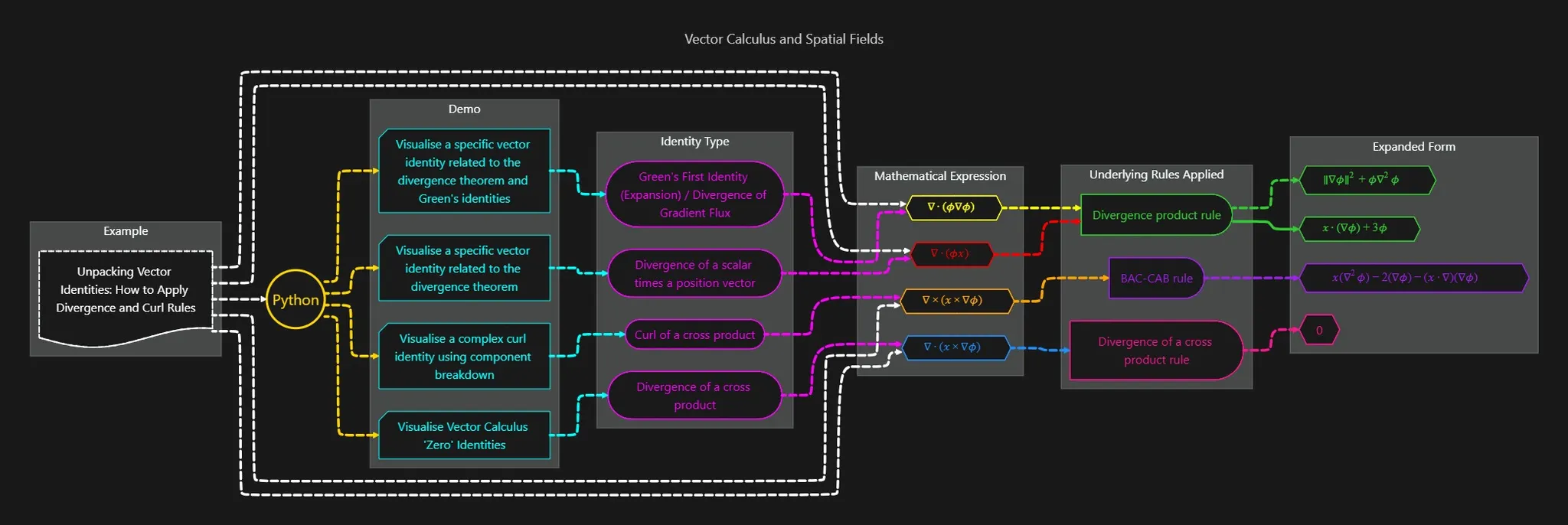
This flowchart, titled **"Vector Calculus and Spatial Fields,"** serves as a structured map for unpacking and visualizing specific vector identities using Python. It traces the logic from a general example down to the specific mathematical rules and their expanded forms.
#### **1. The Starting Point: Example & Python Implementation**
The flow begins on the far left with a core **Example** block: *"Unpacking Vector Identities: How to Apply Divergence and Curl Rules."* This leads into a **Python** node, indicating that the following processes are computational demonstrations or visualizations of these mathematical concepts.
#### **2. Demo & Identity Types**
The Python node branches into four specific **Demos**, each paired with a corresponding **Identity Type**:
| **Demo Objective** | **Identity Type** |
| --------------------------------------------------------------------- | ------------------------------------------------------------------ |
| Visualize identity related to Divergence Theorem & Green's Identities | **Green's First Identity** (Expansion/Divergence of Gradient Flux) |
| Visualize identity related to Divergence Theorem | **Divergence of a scalar times a position vector** |
| Visualize complex curl identity using component breakdown | **Curl of a cross product** |
| Visualize Vector Calculus 'Zero' Identities | **Divergence of a cross product** |
#### **3. Mathematical Expressions & Underlying Rules**
Once the identity type is defined, the chart moves into the **Mathematical Expression** and the **Underlying Rules Applied** to solve or expand them:
* $$\nabla \cdot (\phi \nabla \phi)$$: Uses the **Divergence product rule**.
* $$\nabla \cdot (\phi \mathbf{x})$$: Also utilizes the **Divergence product rule**.
* $$\nabla \times (\mathbf{x} \times \nabla \phi)$$: Employs the **BAC-CAB rule** (a common mnemonic for triple products).
* $$\nabla \cdot (\mathbf{x} \times \nabla \phi)$$: Applies the **Divergence of a cross product rule**.
#### **4. Expanded Form (The Result)**
The final stage on the right shows the **Expanded Form** of these operations:
* $$|\nabla \phi|^2 + \phi \nabla^2 \phi$$ (Resulting from Green's First Identity).
* $$\mathbf{x} \cdot (\nabla \phi) + 3\phi$$ (Resulting from the scalar/position vector divergence).
* $$\mathbf{x}(\nabla^2 \phi) - 2(\nabla \phi) - (\mathbf{x} \cdot \nabla)(\nabla \phi)$$ (Resulting from the complex curl identity).
* **0** (Confirming the 'Zero' identity for the divergence of that specific cross product).
***
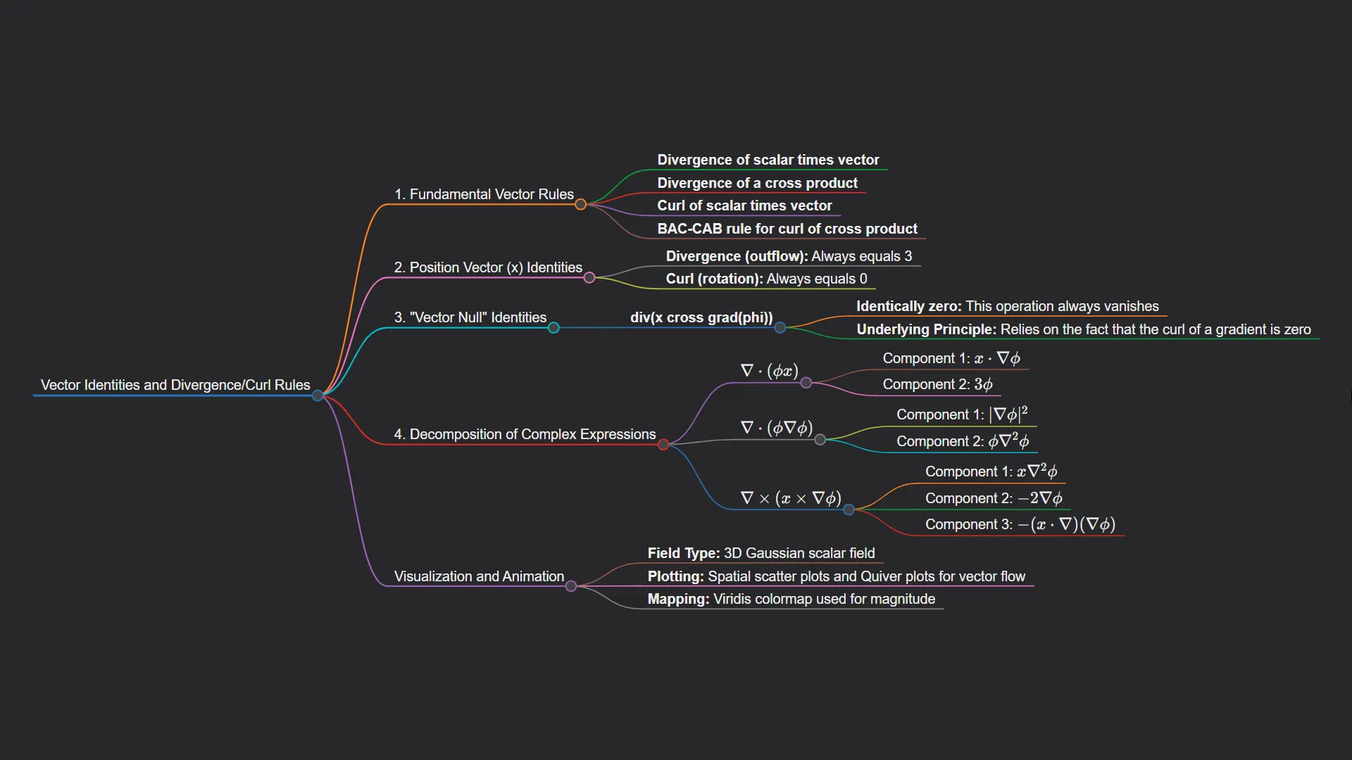
### 📌Vector Identities and Divergence/Curl Rules
Description
This mind map, titled **"Vector Identities and Divergence/Curl Rules,"** provides a structured breakdown of vector calculus principles, their mathematical decomposition, and their computational visualization.
#### **1. Fundamental Vector Rules**
This branch lists the foundational operations used to manipulate vector fields:
* **Divergence of scalar times vector**.
* **Divergence of a cross product**.
* **Curl of scalar times vector**.
* **BAC-CAB rule** for the curl of a cross product.
#### **2. Position Vector (x) Identities**
Focuses on the properties of the position vector field:
* **Divergence (outflow):** Noted as always equaling **3**.
* **Curl (rotation):** Noted as always equaling **0**.
#### **3. "Vector Null" Identities**
Explores expressions that resolve to zero:
* **Operation:** $$div(x \times grad(\phi))$$.
* **Outcome:** It is **identically zero**, meaning the operation always vanishes.
* **Underlying Principle:** It relies on the mathematical fact that the curl of a gradient is zero.
#### **4. Decomposition of Complex Expressions**
This section breaks down specific identities into their constituent mathematical components:
* $$\nabla \cdot (\phi x)$$**:** Decomposes into $$x \cdot \nabla \phi$$ and $$3\phi$$.
* $$\nabla \cdot (\phi \nabla \phi)$$**:** Decomposes into $$|\nabla \phi|^2$$ and $$\phi \nabla^2 \phi$$.
* $$\nabla \times (x \times \nabla \phi)$$**:** Decomposes into three components: $$x \nabla^2 \phi$$, $$-2\nabla \phi$$, and $$-(x \cdot \nabla)(\nabla \phi)$$.
#### **5. Visualization and Animation**
The final branch outlines how these fields are rendered computationally:
* **Field Type:** Utilizes a **3D Gaussian scalar field**.
* **Plotting:** Employs **spatial scatter plots** and **Quiver plots** to represent vector flow.
* **Mapping:** Uses the **Viridis colormap** to indicate magnitude.
### :scarf:Narrated Video
{% embed url="" %}
### :thread:Related Derivation
{% content-ref url="../proof-and-derivation/unpacking-vector-identities-how-to-apply-divergence-and-curl-rules-vi-dcr" %}
[unpacking-vector-identities-how-to-apply-divergence-and-curl-rules-vi-dcr](https://via-dean.gitbook.io/all/~/revisions/WYsapCOkHSgcDPhymfq8/multifaceted-viewpoint/mathematical-structures-underlying-physical-laws/proof-and-derivation/unpacking-vector-identities-how-to-apply-divergence-and-curl-rules-vi-dcr)
{% endcontent-ref %}
### :hammer\_pick:Compound Page
{% embed url="" %}